Worksheet 12.1: Problem 5

5. Assuming the core temperature, \(T_{c}\), is pretty much constant (nuclear fusion is a threshold process with a steep temperature dependence on the reaction rate), what are the following relationships?

Before we start finding these stellar scaling relationships, we need to come up with some scaling relationships from our known differential equations.
\[\frac{dP}{dr}\:=\:-\frac{GM(r)\rho (r)}{r^{2}}\:\rightarrow\:P_{c}\:\sim\:\frac{M^{2}}{R^{4}}\]
\[\frac{dT}{dr}\:=\:-\frac{3L\kappa \rho (r)}{16\pi acT^{3}r^{2}}\:\rightarrow\:T_{c}^{4}\:\sim\:\frac{LM}{R^{4}}\]
\[\frac{dM}{dR}\:=\:4\pi r^{2} \rho (r)\:\rightarrow\:\rho\:\sim\:\frac{M}{R^{3}}\]

These scaling relationships will be used to arrive at our desired scaling relationships in the following problems.

a) Mass-radius (i.e. assume \(R\:\sim\:M^{\alpha}\) and find \(\alpha\))
Since our idealized stars are made entirely of hydrogen gas, we can assume that the Ideal Gas Law applies. The Ideal Gas Law can be written as \(P\:=\:\frac{\rho}{m}kT\:\rightarrow\:P_{c}\:\sim\:\rho T\). We can then plug this into our first scaling relationship:
\[P_{c}\:\sim\:\frac{M^{2}}{R^{4}}\]
\[\rho T_{c}\:\sim\:\frac{M^{2}}{R^{4}}\]
Now using our third scaling relationship, we can substitute for density:
\[\frac{M}{R^{3}}T_{c}\:\sim\:\frac{M^{2}}{R^{4}}\:\rightarrow\:T_{c}\:\sim\:\frac{M}{R}\]
Now assuming a constant \(T_{c}\) in main sequence stars:
\[M\:\sim\:R\]

b) Mass-luminosity (\(L\:\sim\:M^{\alpha}\) for stars with a mass greater than that of the sun, assuming the opacity is independent of temperature. 

Using the scaling relationship found for \(T_{c}\) found in the previous part, we can substitute into our second scaling relationship.
\[T_{c}^{4}\:\sim\:\frac{LM}{R^{4}}\]
\[\frac{M^{4}}{R^{4}}\:\sim\:\frac{LM}{R^{4}}\]
\[L\:\sim\:M^{3}\]

Thus, for high mass stars, luminosity scales with mass cubed.

c) Mass-luminosity for stars with a mass less than or equal to that of the Sun, assuming the opacity scales as \(\kappa\:\sim\:\rho T^{-3.5}\).
Since opacity is no longer assumed to be constant, we have to go back and adjust our derivation for the second scaling relationship to account for the non-constant \(\kappa\). We know that:
\[T_{c}\:\sim\:\frac{L\kappa M}{T_{c}^{3}R^{4}}\:\rightarrow\:\sim\:\frac{L\rho M}{T_{c}^{6.5} R^{4}}\]
Since we know that T_{c} is assumed to be constant and that R scales with M, we can simplify this to:
\[L\:\sim\:M^{5}\]
This scaling relationship holds for less massive stars.

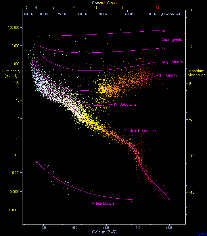
d)   Luminosity-effective temperature for the two mass regimes above.  The locus of points the T-L plane is the so-called Hertzsprung-Russell (H-R) diagram.  Sketch this as log L on the y-axis, and the log Teff running backwards on the x-axis.  Include numbers on each axis over a range of two orders of magnitude in stellar mass (0.1<M<10∗M⊙).  For your blog post, look up a sample H-R diagram showing real data using Google Images.  How does the slope of the observed H-R diagram compare to yours?


In the past few problems, our scaling relationships have used the core temperature rather than the effective temperature. In order to find this scaling relationship, we need to start with an expression that includes the effective temperature. We can use our original expression for luminosity, \(L\:=\:4 \pi R^{2} \sigma T_{eff}^{4}\). Converting this to a scaling relationship gives: \(L\:\sim\:R^{2}T_{eff}^{4}\). In the past two parts of the problem we came up for luminosity scaling relationships for two different stellar mass classifications. If we take the average of these two stellar relationships, we find that \(L\:\sim\:M^{4}\). Since \(M\:\sim\:R\), we can substitute in and get \(L\:\sim\:R^{4}\). We can now use this to substitute into our relationship derived from the original luminosity equation:
\[L\:\sim\:R^{2}T_{eff}^{4}\]
\[L\:\sim\:L^{0.5} T_{eff}^{4}\]
\[L^{0.5}\:\sim\: T_{eff}^{4}\]
\[L\:\sim\:T_{eff}^{8}\]

We can take the log of both sides of this equation and plot it with the log of L on the vertical axis and the log of T on the horizontal axis with \(log(T)\:=\:0\) towards the right of the horizontal axis and becoming larger as you move leftward.

As you can see, this curve is very similar to the actual H-R diagram.